Usuario:Orendona/Taller1

En matemáticas, la transformada de Fourier de tiempo discreto, discrete-time Fourier transform (DTFT) es una forma de en:Fourier analysis that is applicable to a sequence of values.

The DTFT is often used to analyze samples of a continuous function. The term discrete-time refers to the fact that the transform operates on discrete data, often samples whose interval has units of time. From uniformly spaced samples it produces a function of frequency that is a periodic summation of the continuous Fourier transform of the original continuous function. Under certain theoretical conditions, described by the sampling theorem, the original continuous function can be recovered perfectly from the DTFT and thus from the original discrete samples. The DTFT itself is a continuous function of frequency, but discrete samples of it can be readily calculated via the discrete Fourier transform (DFT) (see Plantilla:Slink), which is by far the most common method of modern Fourier analysis.

Both transforms are invertible. The inverse DTFT is the original sampled data sequence. The inverse DFT is a periodic summation of the original sequence. The fast Fourier transform (FFT) is an algorithm for computing one cycle of the DFT, and its inverse produces one cycle of the inverse DFT.

Definition

The discrete-time Fourier transform of a discrete sequence of real or complex numbers x[n], for all integers n, is a Fourier series, which produces a periodic function of a frequency variable. When the frequency variable, ω, has normalized units of radians/sample, the periodicity is 2π, and the Fourier series is:​

$X_{2\pi }(\omega )=\sum _{n=-\infty }^{\infty }x[n]\,e^{-i\omega n}.$ (Eq.1)

The utility of this frequency domain function is rooted in the Poisson summation formula. Let X(f) be the Fourier transform of any function, x(t), whose samples at some interval T (seconds) are equal (or proportional) to the x[n] sequence, i.e. T⋅x(nT) = x[n].​  Then the periodic function represented by the Fourier series is a periodic summation of X(f) in terms of frequency f in hertz (cycles/sec):Plantilla:Efn-la

$X_{1/T}(f)=X_{2\pi }(2\pi fT)\ \triangleq \sum _{n=-\infty }^{\infty }\underbrace {T\cdot x(nT)} _{x[n]}\ e^{-i2\pi fTn}\;{\stackrel {\mathrm {Poisson\;f.} }{=}}\;\sum _{k=-\infty }^{\infty }X\left(f-k/T\right).$ (Eq.2)

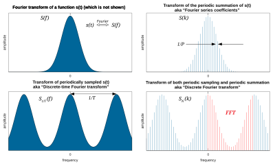
Fig 1. Depiction of a Fourier transform (upper left) and its periodic summation (DTFT) in the lower left corner. The lower right corner depicts samples of the DTFT that are computed by a discrete Fourier transform (DFT).

The integer k has units of cycles/sample, and 1/T is the sample-rate, f_s (samples/sec). So X_1/T(f) comprises exact copies of X(f) that are shifted by multiples of f_s hertz and combined by addition. For sufficiently large f_s the k = 0 term can be observed in the region [−f_s/2, f_s/2] with little or no distortion (aliasing) from the other terms. In Fig.1, the extremities of the distribution in the upper left corner are masked by aliasing in the periodic summation (lower left).

We also note that e^−i2πfTn is the Fourier transform of δ(t − nT). Therefore, an alternative definition of DTFT is:

$X_{1/T}(f)={\mathcal {F}}\left\{\sum _{n=-\infty }^{\infty }x[n]\cdot \delta (t-nT)\right\}.$ (Eq.3)

The modulated Dirac comb function is a mathematical abstraction sometimes referred to as impulse sampling.​

Inverse transform

An operation that recovers the discrete data sequence from the DTFT function is called an inverse DTFT. For instance, the inverse continuous Fourier transform of both sides of Eq.3 produces the sequence in the form of a modulated Dirac comb function:

$\sum _{n=-\infty }^{\infty }x[n]\cdot \delta (t-nT)={\mathcal {F}}^{-1}\left\{X_{1/T}(f)\right\}\ \triangleq \int _{-\infty }^{\infty }X_{1/T}(f)\cdot e^{i2\pi ft}df.$

However, noting that X_1/T(f) is periodic, all the necessary information is contained within any interval of length 1/T. In both Eq.1 and Eq.2, the summations over n are a Fourier series, with coefficients x[n]. The standard formulas for the Fourier coefficients are also the inverse transforms:

${\begin{aligned}x[n]&=T\int _{\frac {1}{T}}X_{1/T}(f)\cdot e^{i2\pi fnT}df\quad \scriptstyle {{\text{(integral over any interval of length }}1/T{\textrm {)}}}\\\displaystyle &={\frac {1}{2\pi }}\int _{2\pi }X_{2\pi }(\omega )\cdot e^{i\omega n}d\omega \quad \scriptstyle {{\text{(integral over any interval of length }}2\pi {\textrm {)}}}\end{aligned}}$ (Eq.4)

Periodic data

When the input data sequence x[n] is N-periodic, Eq.2 can be computationally reduced to a discrete Fourier transform (DFT), because:

• All the available information is contained within N samples.
• X_1/T(f) converges to zero everywhere except at integer multiples of 1/(NT), known as harmonic frequencies. At those frequencies, the DTFT diverges at different frequency-dependent rates. And those rates are given by the DFT of one cycle of the x[n] sequence.
• The DTFT is periodic, so the maximum number of unique harmonic amplitudes is (1/T) / (1/(NT)) = N

The DFT coefficients are given by:

$X[k]\triangleq \underbrace {\sum _{N}x(nT)\cdot e^{-i2\pi {\frac {k}{N}}n}} _{\text{any n-sequence of length N}},$     and the DTFT is:

$X_{1/T}(f)={\frac {1}{N}}\sum _{k=-\infty }^{\infty }X[k]\cdot \delta \left(f-{\frac {k}{NT}}\right).$      Plantilla:Efn-la

Substituting this expression into the inverse transform formula confirms:

$\int _{\frac {1}{T}}X_{1/T}(f)\cdot e^{i2\pi fnT}df\ =\ {\frac {1}{N}}\underbrace {\sum _{N}X[k]\cdot e^{i2\pi {\frac {n}{N}}k}} _{\text{any k-sequence of length N}}\ \equiv \ x(nT),\quad n\in \mathbb {Z} \,$ (all integers)

as expected. The inverse DFT in the line above is sometimes referred to as a Discrete Fourier series (DFS).​

Sampling the DTFT

When the DTFT is continuous, a common practice is to compute an arbitrary number of samples (N) of one cycle of the periodic function X_1/T: ​

${\begin{aligned}\underbrace {X_{1/T}\left({\frac {k}{NT}}\right)} _{X_{k}}&=\sum _{n=-\infty }^{\infty }x[n]\cdot e^{-i2\pi {\frac {k}{N}}n}\quad \quad k=0,\dots ,N-1\\&=\underbrace {\sum _{N}x_{_{N}}[n]\cdot e^{-i2\pi {\frac {k}{N}}n},} _{\text{DFT}}\quad \scriptstyle {{\text{(sum over any }}n{\text{-sequence of length }}N)}\end{aligned}}$

where $x_{_{N}}$ is a periodic summation:

$x_{_{N}}[n]\ \triangleq \ \sum _{m=-\infty }^{\infty }x[n-mN].$     (see Discrete Fourier series)

The $x_{_{N}}$ sequence is the inverse DFT. Thus, our sampling of the DTFT causes the inverse transform to become periodic. The array of ² values is known as a periodogram, and the parameter N is called NFFT in the Matlab function of the same name.​

In order to evaluate one cycle of $x_{_{N}}$ numerically, we require a finite-length x[n] sequence. For instance, a long sequence might be truncated by a window function of length L resulting in three cases worthy of special mention. For notational simplicity, consider the x[n] values below to represent the values modified by the window function.

Case: Frequency decimation. L = N ⋅ I, for some integer I (typically 6 or 8)

A cycle of $x_{_{N}}$ reduces to a summation of I segments of length N.  The DFT then goes by various names, such as:

• window-presum FFT​
• Weight, overlap, add (WOLA)​​​​​​

• polyphase DFT​​
• polyphase filter bank​
• multiple block windowing and time-aliasing.​

Recall that decimation of sampled data in one domain (time or frequency) produces overlap (sometimes known as aliasing) in the other, and vice versa. Compared to an L-length DFT, the $x_{_{N}}$ summation/overlap causes decimation in frequency,​ leaving only DTFT samples least affected by spectral leakage. That is usually a priority when implementing an FFT filter-bank (channelizer). With a conventional window function of length L, scalloping loss would be unacceptable. So multi-block windows are created using FIR filter design tools.​​  Their frequency profile is flat at the highest point and falls off quickly at the midpoint between the remaining DTFT samples. The larger the value of parameter I, the better the potential performance.

Case: L = N+1.

When a symmetric, L-length window function ($x$) is truncated by 1 coefficient it is called periodic or DFT-even. The truncation affects the DTFT.  A DFT of the truncated sequence samples the DTFT at frequency intervals of 1/N. To sample $x$ at the same frequencies, for comparison, the DFT is computed for one cycle of the periodic summation, $x_{_{N}}.$

Fig 2. DFT of e^i2πn/8 for L = 64 and N = 256

Fig 3. DFT of e^i2πn/8 for L = 64 and N = 64

Case: Frequency interpolation. L ≤ N

In this case, the DFT simplifies to a more familiar form:

$X_{k}=\sum _{n=0}^{N-1}x[n]\cdot e^{-i2\pi {\frac {k}{N}}n}.$

In order to take advantage of a fast Fourier transform algorithm for computing the DFT, the summation is usually performed over all N terms, even though N − L of them are zeros. Therefore, the case L < N is often referred to as zero-padding.

Spectral leakage, which increases as L decreases, is detrimental to certain important performance metrics, such as resolution of multiple frequency components and the amount of noise measured by each DTFT sample. But those things don't always matter, for instance when the x[n] sequence is a noiseless sinusoid (or a constant), shaped by a window function. Then it is a common practice to use zero-padding to graphically display and compare the detailed leakage patterns of window functions. To illustrate that for a rectangular window, consider the sequence:

$x[n]=e^{i2\pi {\frac {1}{8}}n},\quad$ and $L=64.$

Figures 2 and 3 are plots of the magnitude of two different sized DFTs, as indicated in their labels. In both cases, the dominant component is at the signal frequency: f = 1/8 = 0.125. Also visible in Fig 2 is the spectral leakage pattern of the L = 64 rectangular window. The illusion in Fig 3 is a result of sampling the DTFT at just its zero-crossings. Rather than the DTFT of a finite-length sequence, it gives the impression of an infinitely long sinusoidal sequence. Contributing factors to the illusion are the use of a rectangular window, and the choice of a frequency (1/8 = 8/64) with exactly 8 (an integer) cycles per 64 samples. A Hann window would produce a similar result, except the peak would be widened to 3 samples (see DFT-even Hann window).

Convolution

The convolution theorem for sequences is:

$x*y\ =\ \scriptstyle {\rm {DTFT}}^{-1}\displaystyle \left[\scriptstyle {\rm {DTFT}}\displaystyle \{x\}\cdot \scriptstyle {\rm {DTFT}}\displaystyle \{y\}\right].$​Plantilla:Efn-la

An important special case is the circular convolution of sequences x and y defined by $x_{_{N}}*y,$ where $x_{_{N}}$ is a periodic summation. The discrete-frequency nature of $\scriptstyle {\rm {DTFT}}\displaystyle \{x_{_{N}}\}$ means that the product with the continuous function $\scriptstyle {\rm {DTFT}}\displaystyle \{y\}$ is also discrete, which results in considerable simplification of the inverse transform:

$x_{_{N}}*y\ =\ \scriptstyle {\rm {DTFT}}^{-1}\displaystyle \left[\scriptstyle {\rm {DTFT}}\displaystyle \{x_{_{N}}\}\cdot \scriptstyle {\rm {DTFT}}\displaystyle \{y\}\right]\ =\ \scriptstyle {\rm {DFT}}^{-1}\displaystyle \left[\scriptstyle {\rm {DFT}}\displaystyle \{x_{_{N}}\}\cdot \scriptstyle {\rm {DFT}}\displaystyle \{y_{_{N}}\}\right].$​​

For x and y sequences whose non-zero duration is less than or equal to N, a final simplification is:

$x_{_{N}}*y\ =\ \scriptstyle {\rm {DFT}}^{-1}\displaystyle \left[\scriptstyle {\rm {DFT}}\displaystyle \{x\}\cdot \scriptstyle {\rm {DFT}}\displaystyle \{y\}\right].$

The significance of this result is explained at Circular convolution and Fast convolution algorithms.

Symmetry properties

When the real and imaginary parts of a complex function are decomposed into their even and odd parts, there are four components, denoted below by the subscripts RE, RO, IE, and IO. And there is a one-to-one mapping between the four components of a complex time function and the four components of its complex frequency transform:​

${\begin{aligned}{\mathsf {Time\ domain}}\quad &\ x\quad &=\quad &x_{_{RE}}\quad &+\quad &x_{_{RO}}\quad &+\quad i\ &x_{_{IE}}\quad &+\quad &\underbrace {i\ x_{_{IO}}} \\&{\Bigg \Updownarrow }{\mathcal {F}}&&{\Bigg \Updownarrow }{\mathcal {F}}&&\ \ {\Bigg \Updownarrow }{\mathcal {F}}&&\ \ {\Bigg \Updownarrow }{\mathcal {F}}&&\ \ {\Bigg \Updownarrow }{\mathcal {F}}\\{\mathsf {Frequency\ domain}}\quad &X\quad &=\quad &X_{RE}\quad &+\quad &\overbrace {i\ X_{IO}} \quad &+\quad i\ &X_{IE}\quad &+\quad &X_{RO}\end{aligned}}$

From this, various relationships are apparent, for example:

• The transform of a real-valued function (xPlantilla:Sub+ xPlantilla:Sub) is the even symmetric function XPlantilla:Sub+ i XPlantilla:Sub. Conversely, an even-symmetric transform implies a real-valued time-domain.
• The transform of an imaginary-valued function (i xPlantilla:Sub+ i xPlantilla:Sub) is the odd symmetric function XPlantilla:Sub+ i XPlantilla:Sub, and the converse is true.
• The transform of an even-symmetric function (xPlantilla:Sub+ i xPlantilla:Sub) is the real-valued function XPlantilla:Sub+ XPlantilla:Sub, and the converse is true.
• The transform of an odd-symmetric function (xPlantilla:Sub+ i xPlantilla:Sub) is the imaginary-valued function i XPlantilla:Sub+ i XPlantilla:Sub, and the converse is true.

Relationship to the Z-transform

$X_{2\pi }(\omega )$ is a Fourier series that can also be expressed in terms of the bilateral Z-transform.  I.e.:

$X_{2\pi }(\omega )=\left.{\widehat {X}}(z)\,\right|_{z=e^{i\omega }}={\widehat {X}}(e^{i\omega }),$

where the ${\widehat {X}}$ notation distinguishes the Z-transform from the Fourier transform. Therefore, we can also express a portion of the Z-transform in terms of the Fourier transform:

${\begin{aligned}{\widehat {X}}(e^{i\omega })&=\ X_{1/T}\left({\tfrac {\omega }{2\pi T}}\right)\ =\ \sum _{k=-\infty }^{\infty }X\left({\tfrac {\omega }{2\pi T}}-k/T\right)\\&=\sum _{k=-\infty }^{\infty }X\left({\tfrac {\omega -2\pi k}{2\pi T}}\right).\end{aligned}}$

Note that when parameter T changes, the terms of $X_{2\pi }(\omega )$ remain a constant separation $2\pi$ apart, and their width scales up or down. The terms of X_1/T(f) remain a constant width and their separation 1/T scales up or down.

Table of discrete-time Fourier transforms

Some common transform pairs are shown in the table below. The following notation applies:

• $\omega =2\pi fT$ is a real number representing continuous angular frequency (in radians per sample). ($f$ is in cycles/sec, and $T$ is in sec/sample.) In all cases in the table, the DTFT is 2π-periodic (in $\omega$).
• $X_{2\pi }(\omega )$ designates a function defined on $-\infty <\omega <\infty$.
• $X_{o}(\omega )$ designates a function defined on $-\pi <\omega \leq \pi$, and zero elsewhere. Then:

$X_{2\pi }(\omega )\ \triangleq \sum _{k=-\infty }^{\infty }X_{o}(\omega -2\pi k).$

• $\delta (\omega )$ is the Dirac delta function
• $\operatorname {sinc} (t)$ is the normalized sinc function
• $\operatorname {rect} (t)$ is the rectangle function
• $\operatorname {tri} (t)$ is the triangle function
• n is an integer representing the discrete-time domain (in samples)
• $u[n]$ is the discrete-time unit step function
• $\delta [n]$ is the Kronecker delta $\delta _{n,0}$

Time domain x[n]	Frequency domain X2π(ω)	Remarks	Reference
$\delta [n]$	$X_{2\pi }(\omega )=1$		​
$\delta [n-M]$	$X_{2\pi }(\omega )=e^{-i\omega M}$	integer $M$
$\sum _{m=-\infty }^{\infty }\delta [n-Mm]\!$	$X_{2\pi }(\omega )=\sum _{m=-\infty }^{\infty }e^{-i\omega Mm}={\frac {2\pi }{M}}\sum _{k=-\infty }^{\infty }\delta \left(\omega -{\frac {2\pi k}{M}}\right)\,$ $X_{o}(\omega )={\frac {2\pi }{M}}\sum _{k=-(M-1)/2}^{(M-1)/2}\delta \left(\omega -{\frac {2\pi k}{M}}\right)\,$     odd M $X_{o}(\omega )={\frac {2\pi }{M}}\sum _{k=-M/2+1}^{M/2}\delta \left(\omega -{\frac {2\pi k}{M}}\right)\,$     even M	integer $M>0$
$u[n]$	$X_{2\pi }(\omega )={\frac {1}{1-e^{-i\omega }}}+\pi \sum _{k=-\infty }^{\infty }\delta (\omega -2\pi k)\!$ $X_{o}(\omega )={\frac {1}{1-e^{-i\omega }}}+\pi \cdot \delta (\omega )\!$	The $1/(1-e^{-i\omega })$ term must be interpreted as a distribution in the sense of a Cauchy principal value around its poles at $\omega =2\pi k$.
$a^{n}u[n]$	$X_{2\pi }(\omega )={\frac {1}{1-ae^{-i\omega }}}\!$	$0<|a|<1$	​
$e^{-ian}$	$X_{o}(\omega )=2\pi \cdot \delta (\omega +a),$     -π < a < π $X_{2\pi }(\omega )=2\pi \sum _{k=-\infty }^{\infty }\delta (\omega +a-2\pi k)$	real number $a$
$\cos(a\cdot n)$	$X_{o}(\omega )=\pi \left[\delta \left(\omega -a\right)+\delta \left(\omega +a\right)\right],$ $X_{2\pi }(\omega )\ \triangleq \sum _{k=-\infty }^{\infty }X_{o}(\omega -2\pi k)$	real number $a$ with $-\pi <a<\pi$
$\sin(a\cdot n)$	$X_{o}(\omega )={\frac {\pi }{i}}\left[\delta \left(\omega -a\right)-\delta \left(\omega +a\right)\right]$	real number $a$ with $-\pi <a<\pi$
$\operatorname {rect} \left[{n-M \over N}\right]$	$X_{o}(\omega )={\sin[N\omega /2] \over \sin(\omega /2)}\,e^{-i\omega M}\!$	integers $M$ and $N$
$\operatorname {sinc} (W(n+a))$	$X_{o}(\omega )={\frac {1}{W}}\operatorname {rect} \left({\omega \over 2\pi W}\right)e^{ia\omega }$	real numbers $W,a$ with $0<W<1$
$\operatorname {sinc} ^{2}(Wn)\,$	$X_{o}(\omega )={\frac {1}{W}}\operatorname {tri} \left({\omega \over 2\pi W}\right)$	real number $W$, $0<W<0.5$
${\begin{cases}0&n=0\\{\frac {(-1)^{n}}{n}}&{\mbox{elsewhere}}\end{cases}}$	$X_{o}(\omega )=j\omega$	it works as a differentiator filter
${\frac {1}{(n+a)}}\left\{\cos[\pi W(n+a)]-\operatorname {sinc} [W(n+a)]\right\}$	$X_{o}(\omega )={\frac {j\omega }{W}}\cdot \operatorname {rect} \left({\omega \over \pi W}\right)e^{ja\omega }$	real numbers $W,a$ with $0<W<1$
${\begin{cases}{\frac {\pi }{2}}&n=0\\{\frac {(-1)^{n}-1}{\pi n^{2}}}&{\mbox{ otherwise}}\end{cases}}$	$X_{o}(\omega )=|\omega |$
${\begin{cases}0;&n{\text{ even}}\\{\frac {2}{\pi n}};&n{\text{ odd}}\end{cases}}$	$X_{o}(\omega )={\begin{cases}j&\omega <0\\0&\omega =0\\-j&\omega >0\end{cases}}$	Hilbert transform
${\frac {C(A+B)}{2\pi }}\cdot \operatorname {sinc} \left[{\frac {A-B}{2\pi }}n\right]\cdot \operatorname {sinc} \left[{\frac {A+B}{2\pi }}n\right]$	$X_{o}(\omega )=$	real numbers $A,B$ complex $C$

Properties

This table shows some mathematical operations in the time domain and the corresponding effects in the frequency domain.

• $*\!$ is the discrete convolution of two sequences
• $x[n]^{*}$ is the complex conjugate of x[n].

Property	Time domain x[n]	Frequency domain $X_{2\pi }(\omega )$	Remarks	Reference
Linearity	$a\cdot x[n]+b\cdot y[n]$	$a\cdot X_{2\pi }(\omega )+b\cdot Y_{2\pi }(\omega )$	complex numbers $a,b$	​
Time reversal / Frequency reversal	$x[-n]$	$X_{2\pi }(-\omega )\!$		​
Time conjugation	$x[n]^{*}$	$X_{2\pi }(-\omega )^{*}\!$		​
Time reversal & conjugation	$x[-n]^{*}$	$X_{2\pi }(\omega )^{*}\!$		​
Real part in time	$\Re {(x[n])}$	${\frac {1}{2}}(X_{2\pi }(\omega )+X_{2\pi }^{*}(-\omega ))$		​
Imaginary part in time	$\Im {(x[n])}$	${\frac {1}{2i}}(X_{2\pi }(\omega )-X_{2\pi }^{*}(-\omega ))$		​
Real part in frequency	${\frac {1}{2}}(x[n]+x^{*}[-n])$	$\Re {(X_{2\pi }(\omega ))}$		​
Imaginary part in frequency	${\frac {1}{2i}}(x[n]-x^{*}[-n])$	$\Im {(X_{2\pi }(\omega ))}$		​
Shift in time / Modulation in frequency	$x[n-k]$	$X_{2\pi }(\omega )\cdot e^{-i\omega k}$	integer k	​
Shift in frequency / Modulation in time	$x[n]\cdot e^{ian}\!$	$X_{2\pi }(\omega -a)\!$	real number $a$	​
Decimation	$x[nM]$	${\frac {1}{M}}\sum _{m=0}^{M-1}X_{2\pi }\left({\tfrac {\omega -2\pi m}{M}}\right)\!$	integer $M$
Time Expansion	$\scriptstyle {\begin{cases}x[n/M]&n={\text{multiple of M}}\\0&{\text{otherwise}}\end{cases}}$	$X_{2\pi }(M\omega )\!$	integer $M$	​
Derivative in frequency	${\frac {n}{i}}x[n]\!$	${\frac {dX_{2\pi }(\omega )}{d\omega }}\!$		​
Integration in frequency	$\!$	$\!$
Differencing in time	$x[n]-x[n-1]\!$	$\left(1-e^{-i\omega }\right)X_{2\pi }(\omega )\!$
Summation in time	$\sum _{m=-\infty }^{n}x[m]\!$	${\frac {1}{\left(1-e^{-i\omega }\right)}}X_{2\pi }(\omega )+\pi X(0)\sum _{k=-\infty }^{\infty }\delta (\omega -2\pi k)\!$
Convolution in time / Multiplication in frequency	$x[n]*y[n]\!$	$X_{2\pi }(\omega )\cdot Y_{2\pi }(\omega )\!$		​
Multiplication in time / Convolution in frequency	$x[n]\cdot y[n]\!$	${\frac {1}{2\pi }}\int _{-\pi }^{\pi }X_{2\pi }(\nu )\cdot Y_{2\pi }(\omega -\nu )d\nu \!$	Periodic convolution	​
Cross correlation	$\rho _{xy}[n]=x[-n]^{*}*y[n]\!$	$R_{xy}(\omega )=X_{2\pi }(\omega )^{*}\cdot Y_{2\pi }(\omega )\!$
Parseval's theorem	$E_{xy}=\sum _{n=-\infty }^{\infty }{x[n]\cdot y[n]^{*}}\!$	$E_{xy}={\frac {1}{2\pi }}\int _{-\pi }^{\pi }{X_{2\pi }(\omega )\cdot Y_{2\pi }(\omega )^{*}d\omega }\!$		​

See also

• Least-squares spectral analysis
• Multidimensional transform
• Zak transform

Notes

Page citations

References

Further reading

• Porat, Boaz (1996). A Course in Digital Signal Processing. John Wiley and Sons. pp. 27-29 and 104-105. ISBN 0-471-14961-6. 
• Siebert, William M. (1986). Circuits, Signals, and Systems. MIT Electrical Engineering and Computer Science Series. Cambridge, MA: MIT Press. ISBN 0262690950. 
• Lyons, Richard G. (2010). Understanding Digital Signal Processing (3rd edición). Prentice Hall. ISBN 978-0137027415.